# Initialize Otter
import otter
grader = otter.Notebook("lab02-bickel-blank.ipynb")
# Run this cell.
from datascience import *
import matplotlib.pyplot as plt
%matplotlib inline
plt.style.use('fivethirtyeight')
import numpy as np
import warnings
warnings.filterwarnings('ignore')Lab 2: Visualization and Simpson’s Paradox
Goals:
Load and inspect real admissions data
Compare overall and department-level admission rates by gender
Visualize Simpson’s Paradox
Dataset Source: The dataset used in this notebook is a cleaned version of the original UC Berkeley 1973 graduate admissions data, processed by the University of Illinois at Urbana-Champaign.
References:
What do you notice?
What do you wonder?
What story does this tell, especially about the community this data may impact?
| Group | Applicants | Admitted | Men Applicants | Men Admitted | Women Applicants | Women Admitted |
|---|---|---|---|---|---|---|
| Total | 12,763 | 41% | 8,442 | 44% | 4,321 | 35% |
| Dept | All Applicants | All Admitted | Men Applicants | Men Admitted | Women Applicants | Women Admitted |
|---|---|---|---|---|---|---|
| A | 1,246 | 73% | 1,138 | 72% | 108 | 82% |
| B | 585 | 63% | 560 | 63% | 25 | 68% |
| C | 918 | 35% | 325 | 37% | 593 | 34% |
| D | 792 | 34% | 417 | 33% | 375 | 35% |
| E | 584 | 25% | 191 | 28% | 393 | 24% |
| F | 714 | 7% | 373 | 6% | 341 | 7% |
| Total | 4,839 | 43% | 3,004 | 50% | 1,835 | 30% |
[Discussion] Visualization Talk
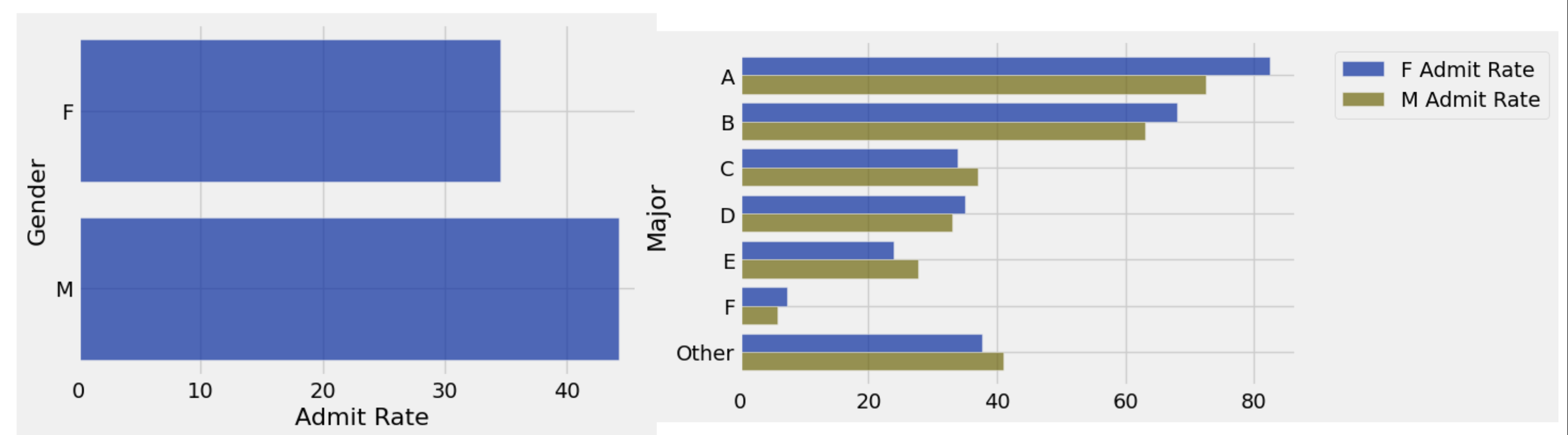
What do you notice?
What do you wonder?
What columns plotted what? (Focus on axes)
[Tutorial] Python the Calculator
The two building blocks of Python code are expressions and statements. An expression is a piece of code that
is self-contained, meaning it would make sense to write it on a line by itself, and
usually evaluates to a value.
The below expression evaluates to 3:
# just run this cell
5 - 2
One important type of expression is the call expression. A call expression begins with the name of a function and is followed by the argument(s) of that function in parentheses. The function returns some value, based on its arguments. For example the function abs returns the absolute value of its argument. The below call expression therefore also evaluates to 3:
# just run this cell
abs(2 - 5)
A statement is a whole line of code. Some statements are just expressions, like the ones above.
Other statements make something happen rather than having a value. For example, an assignment statement assigns a value to a name.
A good way to think about this is that we’re evaluating the right-hand side of the equals sign and assigning it to the left-hand side. Here are some assignment statements:
height = 1.3
the_number_five = abs(-5)
absolute_height_difference = abs(height - 1.688)
An important idea in programming is that large, interesting things can be built by combining many simple, uninteresting things. The key to understanding a complicated piece of code is breaking it down into its simple components.
# if you'd like, copy the lines above into this cell
# and try running it.
Part 1: Table Transformations
[Tutorial] Load the data
Load in the file below by running the cell below.
How is this data different from the tables you analyzed above? How might we build the table above from the one below?
# just run this cell
cal_data = Table.read_table('UCBerkeley1973_Admission.csv')
cal_data.show(5)
We can transform this table in many ways by performing an operation on its rows. Let’s say we wanted all the applicants who were admitted. We can use the table method where:
# just run this cell
cal_data.where("Admission", "Admitted")
[Tutorial] where and num_rows
Now let’s dive into the details a bit more. where takes 2 arguments:
The name of a column.
wherefinds rows where that column’s values meet some criterion.A predicate that describes the criterion that the column needs to meet.
The expression above found all rows whose "Admission" value matched "Admitted". where returns a table that’s a copy of the original table, but with only the rows that meet the given predicate.
To count the number of rows in a table, we can use num_rows. The table property num_rows returns the number of rows in a table. (A “property” is just a method that doesn’t need to be called by adding parentheses.)
Note: The terms “method” and “function” are technically not the same thing, but for the purposes of this course, we will use them interchangeably.
The expression below does many things. Try talking it through with a neighbor, then expand the explanation below.
Explanation
Below, the “equals” sign (
=) assigns the left-hand side name to the value of the right-hand side.The right-hand side:
wherereturns a table that’s a copy of the original table, but only contains rows where the column matches a value, e.g.,"Gender"matches"F".num_rowsgets the numbers of rows that match thewhere.
printis a special function. Theprintexpression displays the values we care about.
# just run this cell
total_f = cal_data.where("Gender", "F").num_rows
print(total_f)
Test your understanding! What do you think the “double” where does below?
Explanation
Since the value of the expression cal_data.where("Admission", "Admitted") is itself a table, you can just call a table method on it.
# just run this cell
total_f = cal_data.where("Gender", "F").num_rows
total_m = cal_data.where("Gender", "M").num_rows
admit_f = cal_data.where("Admission", "Admitted").where("Gender", "F").num_rows #number of female applicants who were accepted
admit_m =  cal_data.where("Admission", "Admitted").where("Gender", "M").num_rows #number of male applicants who were accepted

print(total_f, "total number of female applicants")
print(total_m, "total number of male applicants")
print(admit_f, "number of female applicants admitted")
print(admit_m, "number of male applicants admitted")
Now that we’ve built these values, we can use them in mathematical expressions.
# just run this cell
print(cal_data.num_rows, "number of rows in table")

total = total_f + total_m
print(total, "number of applicants")
Question 1: Compute Admit Rate
Fill in the ... with the given named values
total_ftotal_madmit_f, andadmit_m
to compute the 1973 admission rates (admit rates, in %) for
women (
admit_rate_f) andmen (
admit_rate_m).
NOTE: In Python, / is division, and * is multiplication. How might we compute percentages (between 0 and 100)?
Note 2: If you are encountering an error, raise your hand and we will come by to help.
# TODO: replace the "..." below!
admit_rate_f = ...
admit_rate_m = ...

# do not edit below this line
print("1973's Berkeley admission rate:")
print("female:", admit_rate_f, "%")
print("male:", admit_rate_m, "%")grader.check("q_admit_rates")[Tutorial] .pivot (Berkeley admissions)
Let’s practice one classical table transformation. The pivot method creates a two-way table showing the intersection of two columns.
pivot(columns, rows, values=None, collect=None)
columns: unique values become the new column headersrows: unique values become the row labelsif you do not pass
valuesandcollect, each cell is a count of rows
Example: For this dataset,
columns='Admission'gives columns likeAdmittedandRejectedrows='Gender'gives rows forFandM
So running the below cell builds a table admit_vs_reject that answers:
For each gender, how many applications were admitted vs. rejected?
# just run this cell
admit_vs_reject = cal_data.pivot('Admission', 'Gender')
admit_vs_reject
Question 2: Build count_by_dept
Using the cal_data table loaded earlier and the table method from the section above, complete the cell below to create a table named count_by_dept that shows the number (count) of applicants by Major and Gender. Your count_by_dept table should look like the following:
| Major | F | M |
|---|---|---|
| A | 108 | 1138 |
| B | 25 | 560 |
| C | 593 | 325 |
| D | 375 | 417 |
| E | 393 | 191 |
| F | 341 | 373 |
| Other | 2486 | 5438 |
IMPORTANT NOTE: Use the correct column names as strings. The string of the column names that you want to pass into as the arguments must have the exact match in capitalization, spelling, spaces, etc.
count_by_dept = ...
count_by_deptgrader.check("q_count_by_dept")Question 3: Build admit_by_dept
Recall what we said earlier:
Since the value of the expression
cal_data.where("Admission", "Admitted")is itself a table, you can just call a table method on it.
Now, we know a second table method: pivot...!
Put together what you know about where and pivot to use cal_data to build the admit_by_dept table that shows the number (count) of admits by major and gender. Your admit_by_dept table should look like the following:
| Major | F | M |
|---|---|---|
| A | 89 | 825 |
| B | 17 | 353 |
| C | 201 | 120 |
| D | 131 | 138 |
| E | 94 | 53 |
| F | 25 | 22 |
| Other | 937 | 2227 |
admit_by_dept = ...
admit_by_deptgrader.check("q_admit_by_dept")We will reuse your newly created count_by_dept and admit_by_dept tables later in Part 3’s visualizations with bar charts. For now, you are done with this section, so give yourself a pat on the back!
For those curious, check our the full list of table transformations available in the datascience package.
We’ll circle back for some discussion before we revisit the next part.
Part 3: Bar Charts
The “proper pooling” section of the Simpson’s paradox visualization encodes four variables:
a. Total admits (and rejects) by gender b. Admits (and rejects) by department c. Total admit rate by gender d. Admit rate by department
These can all be visualized with bar charts (one per variable). Let’s tackle (a) and (c) first.
[Tutorial].barh (Berkeley admissions)
Use .barh to make a horizontal bar chart or .bar to make a vertical bar chart from a table with categories.
(horizontal) table.barh(category_column, optional_numeric_columns)
(vertical) table.bar(category_column, optional_numeric_columns)
first argument: the category labels (y-axis)
if no numeric columns are specified,
barhplots all numeric columns
(a) [Tutorial] Plot Total Admits by Gender
Earlier, we built the admit_vs_reject table for you:
# just run this cell
admit_vs_reject
We can use the admit_vs_reject table to plot a (horizontal) bar chart with one horizontal bar for each gender, disaggregated by accepted vs rejected counts.
category column:
Gendernumeric columns:
Admitted,Rejected
# just run this cell
admit_vs_reject.barh("Gender")# just run this cell
admit_by_deptUse the admit_by_dept table to plot the below bar chart.
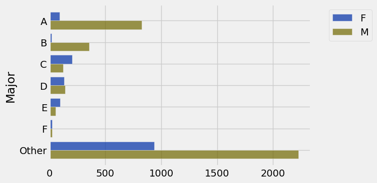
# TODO: write a line below, replacing the ...

...
[Tutorial] Arrays and Tables
How can we add columns to tables? In the datascience library, we can make new columns by creating an array, which is a list of values, in order. Run the cell below and notice that admit_rate is an array with two elements.
admit_rate = make_array(admit_rate_f, admit_rate_m)
admit_rate
An array is not a table, because it doesn’t have labeled columns.
We can add new columns to tables by calling with_columns on that table. The with_columns method requires two arguments:
The name of the first column as a string
An array of values to put in the first column
(optional) The name of the second column as a string
(optional) An array of values to put in the second column
(optional) etc.
For example, the admit_vs_reject_rate table below adds one column to admit_vs_reject; this column is labeled "Admit Rate" and has the values in the admit_rate array.
# just run this cell
admit_vs_reject_rate = admit_vs_reject.with_columns("Admit Rate", admit_rate)
admit_vs_reject_rate
(c) [Tutorial] Plot Acceptance Rates by Gender
We can then use our newly created admit_vs_reject_rate to plot a bar chart of the total admit rates, not the counts as before.
# just run this cell
admit_vs_reject_rate.barh("Gender", "Admit Rate")
[Tutorial] Array Arithmetic
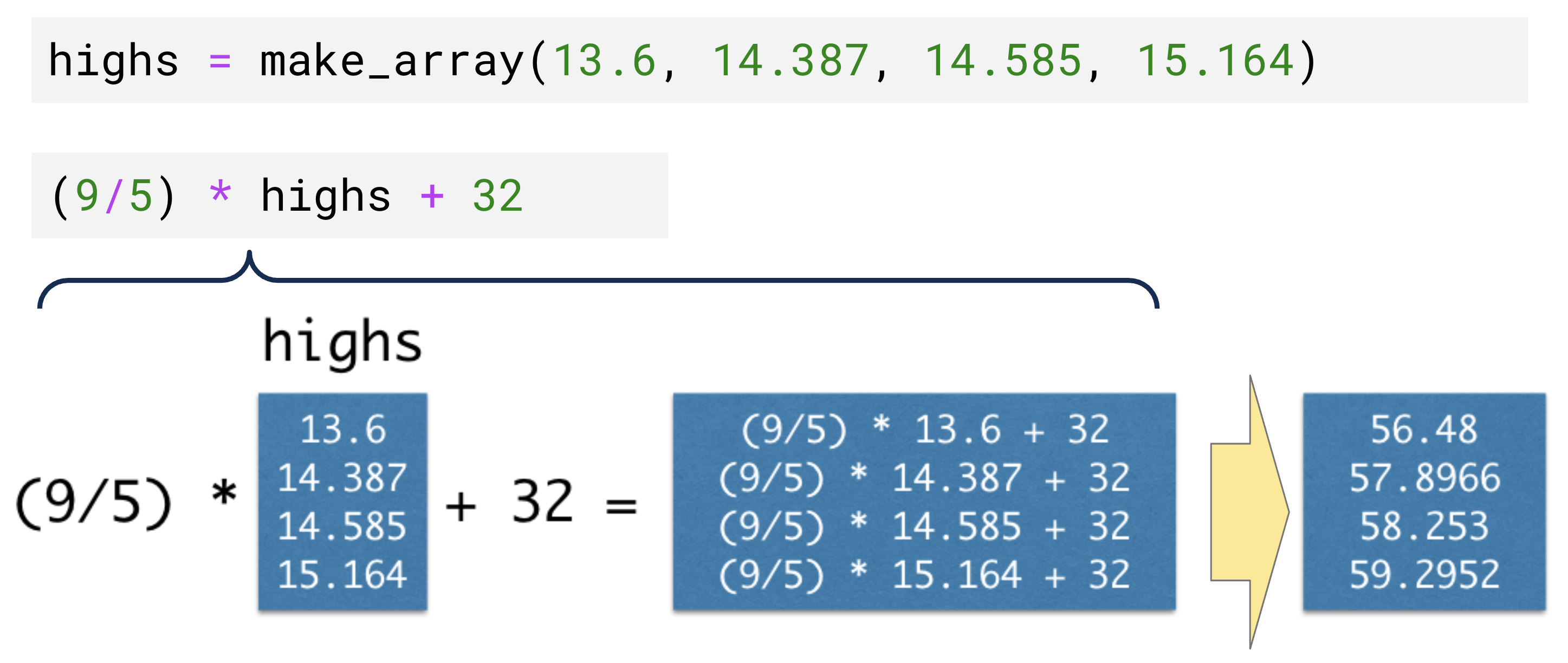
Now we are going to do something really cool: array arithmetic. This is when we use arrays themselves in expressions. When we do so, arithmetic is applied to each element individually.
The cell below illustrates how to use arrays to convert multiple temperatures in Celsius (in the highs array) to Farenheit:
# just run this cell
highs = make_array(13.6, 14.387, 14.585, 15.164)
# just run this cell
(9/5) * highs + 32Below, Table() returns an “empty” table, from which we can add new columns, provided that the number of elements in each column are equal.
# just run this cell. notice the new table...!
Table().with_columns("Celsius", highs,
                     "Farenheit", (9/5) * highs + 32)
Above, we showed how to make columns out of arrays to add to existing tables or make new tables. But what about going the other way?
The column method takes a column label and returns a copy of the values of that column as an array (which, again, is a list of the values in that column, in order). For example, the below cell gets the “M” column in count_by_dept and stores it in m_by_dept:
# just run this cell
m_by_dept = count_by_dept.column("M")
m_by_dept
Since the column method returns arrays, we can now perform array arithmetic “on columns.” The below cell adds the number of male and female applicants by department and stores it in total_by_dept:
# just run this cell
total_by_dept = count_by_dept.column("M") + count_by_dept.column("F")
total_by_dept
Before we introduce the next question, here is a refresher on two tables you have malready built:
# just run this cell
count_by_dept
# just run this cell
admit_by_deptQuestion 5: Compute Admit Rate by Department
Use the two tables count_by_dept and admit_by_dept with the column method to compute admit_f_by_dept_rate and admit_m_by_dept_rate to the admission percentages (between 0 and 100) of female and males to each department, respectively.
If all goes well, then running the cell below should correctly produce admit_by_dept_rate, a table of rates that match what you observed in the Simpson’s website demo.
# TODO: fill in the blanks
admit_f_by_dept_rate = ...
admit_m_by_dept_rate = ...

# do not edit below this line
admit_by_dept_rate = Table().with_columns(
                        "Major", admit_by_dept.column("Major"),
                        "F Admit Rate", admit_f_by_dept_rate,
                        "M Admit Rate", admit_m_by_dept_rate)
admit_by_dept_rategrader.check("q_admit_by_dept_rate")(d) Question 6: Plot Admit Rate by Department
Finally, in the cell below, choose one of the many many tables that we have built over the entire notebook to plot the admit rate by department.
...Submission
Make sure you have run all cells in your notebook in order before running the cell below, so that all images/graphs appear in the output. The cell below will generate a zip file for you to submit. Please save before exporting!
# Save your notebook first, then run this cell to export your submission.
grader.export(pdf=False)- Bickel, P. J., Hammel, E. A., & O’Connell, J. W. (1975). Sex Bias in Graduate Admissions: Data from Berkeley: Measuring bias is harder than is usually assumed, and the evidence is sometimes contrary to expectation. Science, 187(4175), 398–404. 10.1126/science.187.4175.398